Sometimes it might be necessary to understand whether the data you have follows any trend or pattern. The simplest way to understand whether there is a pattern is by fitting a line through data.
Sections
1. Introduction
Line fitting is related to creating a simple linear regression model. Linear means straight line; regression is an analysis that tries to understand the relationship between two or more variables (things that change). The word model means that something is fitted within a more compact explanation of that data (or phenomenon). The beauty of models is that they have predictive powers. For instance, if you observe that the more you travel by car, the more gas you have to spend, a linear model might be just right for you. Once the model has been constructed, you can use it to predict how much gas you will spend per kilometer.
As you might've guessed not all two phenomena follow a linear relationship. For instance, when you practice a skill, at first, you get better fast, however, the longer you practice, the slower you improve. This kind of relationship is called power law of practice (Newell, Rosenbloom, 1981, p.4), or law of diminishing returns.
Things in life, however, are hardly linear. Normally, you can start with a linear model and find out how wrong it is. Then, you can adjust or change it and make it more complex so that it fits the reality and describes the observed phenomena. Still, if you want to have a better understanding about an observation of two phenomena, fitting a line is a good place to start.
2. Theory
Note 1. Skip this part if you want to get straight to coding.
Note 2. This part assumes that you know what a linear function, sigma notation, arithmetic mean, and partial derivatives are. If you don't, I will try to be clear.
First, we’ll need a linear function which will serve as base for our line that fits the data. The canonical form of a linear function is:
$$ \begin{equation} y=a+bx \end{equation} $$
In other words, a line passes through y-axis at the value a (a.k.a. y-intercept), and the slope of that line is b. The letters a and b, in the case of simple linear regression, are merely numbers.
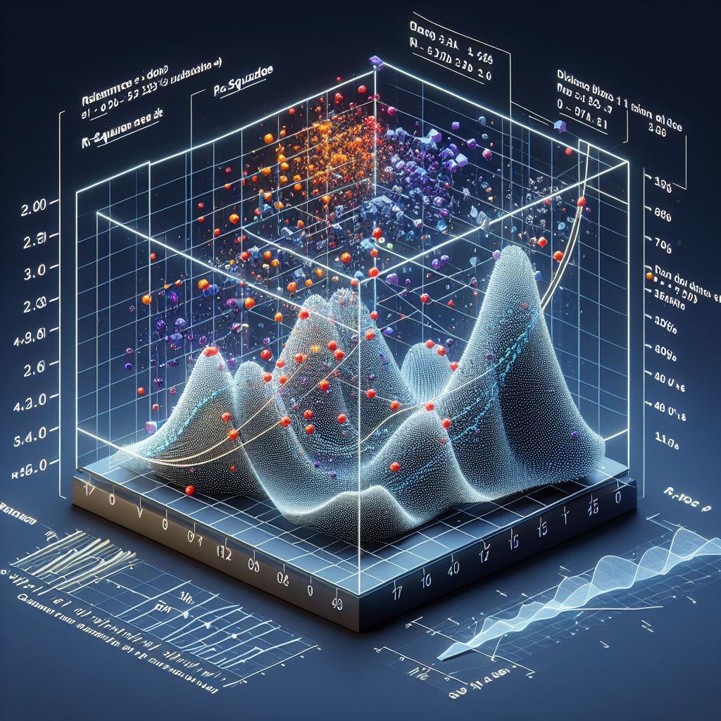
Now, imagine trying to fit a line through a number of data points. After a few trials you’ll find out that there is no single straight line that passes through all the data points. However, since we keep insisting on drawing a line, we need to find one that will be closest to each of the data points. To draw that line, we will need a quantity that we will denote as ε, called epsilon, which will measure the distance from the line to each data point as shown in Figure 1. In statistics that quantity is called error, or prediction error, and it fittingly describes how badly the model explains the data points. Below is an example that illustrates line fitting using error.
Figure 1
Scatter plot of fuel consumption for measured distances
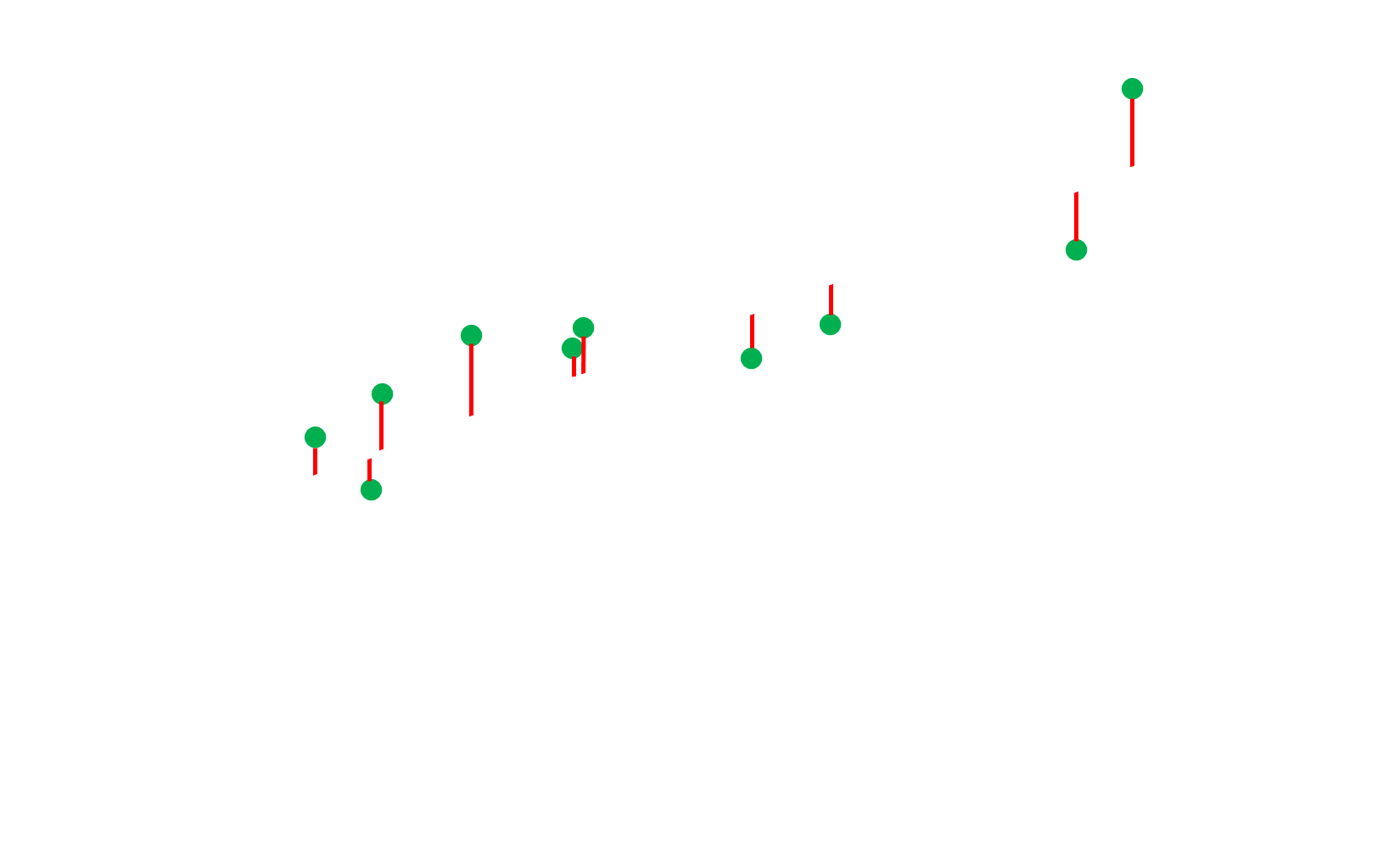
The white line that crosses through the data points is the "trend line" that we're trying to derive mathematically. In other words, the line is graphed based on the model from equation 1. The red lines represent the individual errors and they tell how far off is the model (the line) from the specific data point.
Taking everything into account, we need to update our linear model to include the individual errors:
$$ \begin{equation} y_i=a+bx_i+\epsilon_i \end{equation} $$
Now, let's imagine we have n data points (10 for example), we will denote each of them with an index i (x1, x2, ..., x10). All these data points will be called xi and yi. We will use only x and y, because simple linear regression is done only on two variables. I also made a small change, did you notice it? I added the subscript i to x, y, and ε because we want the error to describe the deviation of the line from each data point.
Rewriting equation 2 in terms of ε,
$$ \begin{equation} \epsilon_i=y_i-a-bx_i \end{equation} $$
Let us also imagine that we have a new function that tells us what is the total error. It will be a sum of all the errors for each data point and we will call it E. It will have two inputs, the y-intercept a and the slope b. E is also called error metric and it describes the fitness of the model; i.e., how well the model describes the data. The smaller the value of E, the the smaller the error, and the greater its fitness.
$$ \begin{equation} E(a,b)=\sum_{i=1}^n(\epsilon_i)^2 \end{equation} $$
$$ \begin{equation} E(a, b)=\sum_{i=1}^n(y_i-a-bx_i)^2 \end{equation} $$
The sigma (Σ) means sum. In the equation 5, E is equal to the sum of all errors. To get the best fitting line it is necessary for E to have the smallest possible value. This can be achieved by varying its input a and b. Go back to Figure 1 and try to move it up and down and change its slope, how does the individual errors change? In this imaginary exercise you tried to vary a and b. In contrast, there is a special and beautiful technique to find the maximum or the minimum of a function, E in this case. To find the minimum of E, we should first find its derivative and then equal it to zero. This can be written as follows:
$$ \begin{equation} \frac{\partial E}{\partial a}=0 \end{equation} $$
$$ \begin{equation} \frac{\partial E}{\partial b}=0 \end{equation} $$
We will start by solving the equation 6.
$$ \frac{\partial E}{\partial a}=\frac{\partial}{\partial a}{\sum_{i=1}^n(\epsilon_i)^2} $$
The summation goes before the partial derivative and epsilon is treated as a function; therefore,
$$ \frac{\partial E}{\partial a}=\sum_{i=1}^n\frac{\partial}{\partial a}(\epsilon_i)^2=2\sum_{i=1}^n {\epsilon_i} \frac{\partial \epsilon_i}{\partial a} $$
Solving the partial derivative of the epsilon,
$$ \frac{\partial \epsilon_i}{\partial a}=\frac{\partial}{\partial a}{(y_i-a-bx_i)}=-1 $$
Substituting the result in the partial derivative of E with respect to a,
$$ \frac{\partial E}{\partial a}=-2\sum_{i=1}^n {(y_i-a-bx_i)} $$
$$ -2\sum_{i=1}^n {(y_i-a-bx_i)} = 0 $$
Since zero divided by anything is zero it can be dropped,
$$ \sum_{i=1}^n {(y_i-a-bx_i)} = 0 $$
Expanding the sum and solving for a:
$$ \sum_{i=1}^n {y_i} - \sum_{i=1}^n {a} - \sum_{i=1}^n {bx_i} = 0 $$
$$ \sum_{i=1}^n {y_i} - na - b\sum_{i=1}^n {x_i} = 0 $$
$$ na = \sum_{i=1}^n {y_i} - b\sum_{i=1}^n {x_i} $$
$$ \begin{equation} a = \frac{\sum_{i=1}^n {y_i} - b\sum_{i=1}^n {x_i}}{n} \end{equation} $$
In order to keep solving we need to do a substitution. First, it will be helpful to remember that the mean value (x with a bar on top) is the sum of all the quantities divided by the amount of those quantities, n. In other words,
$$ \bar{x} = \frac{x_1 + x_2 + x_3 + ... + x_n}{n} $$
Is the same as,
$$ \begin{equation} \bar{x} = \frac{\sum_{i=1}^{n}x_i}{n} \end{equation} $$
Now, we can substitute the mean value formula (9) into the equation 8.
$$ a = \frac{\sum_{i=1}^n {y_i}}{n} - \frac{b\sum_{i=1}^n {x_i}}{n} = \bar{y}-b\bar{x} $$
Here is the clean version of the minimized value of a (y-intercept), we will need it later when we solve the minimized value of b (slope).
$$ \begin{equation} a=\bar{y}-b\bar{x} \end{equation} $$
Now, let’s solve solve the partial derivative of total error E with respect to b.
$$ \frac{\partial E}{\partial b} = \frac{\partial}{\partial b}{\sum_{i=1}^{n}(\epsilon_i)^2} $$
Once again, treating epsilon as an equation yields
$$ \frac{\partial E}{\partial b} = 2\sum_{i=1}^{n}{\epsilon_i}\frac{\partial \epsilon_i}{\partial b} $$
Solving the partial derivative of error with respect to b
$$ \begin{equation} \frac{\partial E}{\partial b} = -2\sum_{i=1}^{n}{x_i(y_i-a-bx_i)} \end{equation} $$
Substituting equation 10 into equation 11:
$$ \frac{\partial E}{\partial b} = -2\sum_{i=1}^{n}{x_i(y_i-(\bar{y}-b\bar{x})-bx_i)} = -2\sum_{i=1}^{n}{x_i(y_i-\bar{y}+b\bar{x}-bx_i)} $$
Making the partial derivative equal to zero as given in equation 7:
$$ -2\sum_{i=1}^{n}{x_i(y_i-\bar{y}+b\bar{x}-bx_i)} = 0 $$
Opening the sums and solving for b:
$$ \sum_{i=1}^{n}{(x_i y_i-x_i\bar{y}+bx_i\bar{x}-bx_i^2)} = 0 $$
$$ \sum_{i=1}^{n}{(x_i y_i-x_i\bar{y})}+b\sum_{i=1}^{n}{x_i\bar{x}-x_i^2)} = 0 $$
$$ b\sum_{i=1}^{n}{(x_i\bar{x}-x_i^2)} = \sum_{i=1}^{n}{(x_i\bar{y}-x_i y_i)} $$
$$ \begin{equation} b = \frac{\sum_{i=1}^{n}{(x_i\bar{y}-x_i y_i)}}{\sum_{i=1}^{n}{(x_i\bar{x}-x_i^2)}} \end{equation} $$
That's it! Quite an adventure. Now, the only thing left is to find data, use the equation 10 and 12 to calculate a and b and substitute then into the model equation (1)
Note 3. Sometimes you might find the formula for b like this: \(b = \frac{\sum_{i=1}^{n}{(x_i-\bar{x})(y_i - \bar{y})}}{\sum_{i=1}^{n}{(x_i-\bar{x})^2}}\), don't worry, they're the same.
3. Practice
Now that we have a model of simple linear regression, we can collect data. Imagine you have a car and you want to measure specifically how much liters of gas it consumes per kilometer.
Below is a sample of the data I have collected.
Table 1
| Distance (km) | Consumption (l) |
|---|---|
| 1.0 | 0.424 |
| 1.6 | 0.51 |
| 2.4 | 0.6256 |
| 1.5 | 0.321 |
| 3.3 | 0.6002 |
| 4.9 | 0.5806 |
| 3.4 | 0.6396 |
| 7.8 | 0.7932 |
| 8.3 | 1.11 |
| 5.6 | 0.6464 |
In fact, the data from the table is plotted in the Figure 1.
The numpy library for Python is a prerequisite and we will rely on it because it has some convenient array operations.
The first thing you have to do is to import the numpy library and create a list with x and y data.
  import numpy as np

  x = np.array([1.0, 1.6, 2.4, 1.5, 3.3, 4.9,\
                3.4, 7.8, 8.3, 5.6])
  y = np.array([0.424, 0.5104, 0.6256, 0.321,\
                0.6002, 0.5806, 0.6396, 0.7932, 1.1102, 0.6464])
We initialize a numpy array with a python built-in list that contains the data from the Table 1. The next step is to calculate the mean of the array x and y. Conveniently, numpy arrays already have a method to calculate the mean.
  meanx = x.mean()
  meany = y.mean()
We’re almost done. We need to calculate the a and b using the equations 10 and 12 respectively. I included them below for convenience.
$$ \begin{align*} a = \bar{y}-b\bar{x}, & \hspace{30px} b = \frac{\sum_{i=1}^{n}{(x_i\bar{y}-x_i y_i)}}{\sum_{i=1}^{n}{(x_i\bar{x}-x_i^2)}} \end{align*} $$
Converting these formulas to python code produces:
b = (x * meany - x * y).sum() / (x * meanx - np.power(x, 2)).sum()
The first thing that should catch our attention is the usage of .sum(). Because x and y is an array, the resulting calculations within the parentheses will also yield a numpy array. That array has the method .sum() that sums all the elements in the array. You might be asking yourself why we didn’t start with equation for the parameter a. The reason is that to calculate the parameter a we need to first calculate the parameter b.
The next step is to calculate the parameter a:
a = meany - b * meanx
The last step is to print these parameters:
print(f'Linear regression model: y = {a:.5f} + {b:.5f}x')
If you run the full code it will output the following:
Linear regression model: y = 0.33896 + 0.07190x
Graphing this model into the Figure 1:
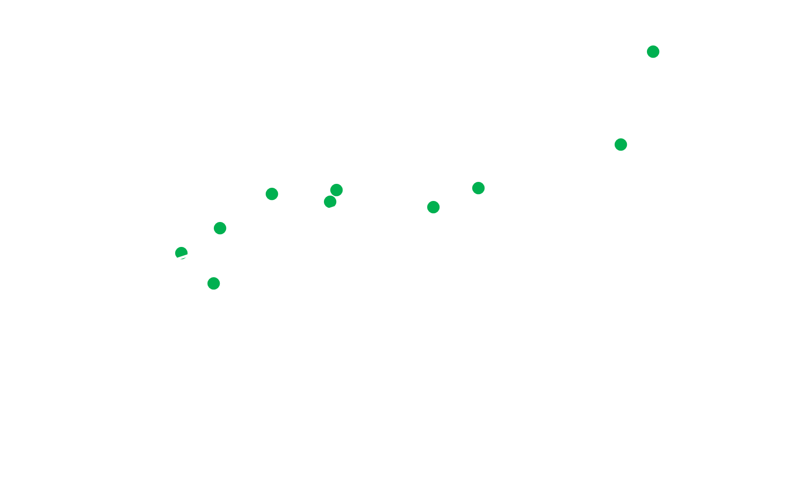
With this model it is also possible to find the fuel-consumption per kilometer, which is the b-value: 0.0719. In other words, the car consumes approximately 0.0719 liters per kilometer.
Going even further we can calculate the strength of this linear relationship. According to a review published in 2013 on statistics (Bewick, Cheek, & Ball, 2003), a quantity that measures the strength of the relationship between two variables (e.g. distance and consumption) is Pearson’s r coefficient. This coefficient can take values between minus and plus one. A coefficient equal to plus one would mean that the linear regression model fits perfectly the data; i.e., the error function is zero. If the coefficient is minus one, that would also mean that the error function is zero and that the model fits the data perfectly; however, it would also mean that when one quantity increases, the other decreases. A Pearson’s coefficient of zero would mean that the error function is maximal and the regression model cannot describe the data.
In practice, it is impossible to get a plus or minus one, or a zero for the coefficient r. The nature forbids it. Its inherent chaos (extraneous variables) always adds noise to the gathered data; in other words, because nothing is perfect in nature (including the measurement instruments) the observed data is modified.
The formula for Pearson’s coefficient r is:
$$ r=\frac{\sum_{i=1}^{n}{(x_i-\bar{x})(y_i-\bar{y})}}{\sqrt{\sum_{i=1}^{n}{(x_i-\bar{x})^2\sum_{i=1}^{n}{(y_i-\bar{y})^2}}}} $$
It looks menacing only on paper. It has the same dividend as the b-value in Note 3 in the Section 2. Let’s write the code to calculate the r.
  r = ((x-meanx) * (y-meany)).sum() \
      / np.sqrt(np.power(x - meanx, 2).sum() \
      * np.power(y - meany, 2).sum())
The r for the fuel-consumption data is 0.872 which is quite good. This number says that the correlation between the observed fuel consumption and the measured distance is 0.872.
You might ask yourself why not use the error metric function, E? The function E allows only for positive values; in other words, it describes the amount of error. Pearson’s r, on the other hand, describes not only the amount of error but also the relationship between the two variables (hence, the interval between minus and plus one).
4. The Hammer and The Butterfly
There is a wonderful phrase which became almost ubiquitous in latest books on machine learning: to a man with a hammer everything is a nail. I think it wonderfully captures the current scientific trend. A momentous quantity of quantitative research papers contain a linear correlation coefficient. There is nothing bad in using linear regression to understand the observed phenomena; however, the problem arises when you limit yourself only to the linear regression. Even sillier is when you flaunt your results and say that there is a linear relationship between two variables. No. It is likely that you used a hammer on a butterfly.
It is important to apply a wide variety of instruments to analyze the data. Even when you want to build a model just as we did above. For instance, some data is exponential, other is polynomial, logistic, or non-existent. Consider this.
It makes sense to use linear modelling for fuel consumption because we can expect the car to use the same amount of fuel whether at the first kilometer or at the ninth. For instance, you can draw a trend (linear regression) on sample market data, but you can’t expect it to reach the moon. Furthermore, it doesn’t make sense to expect your skill to improve ad astra (Newell & Rosenbloom, 1981). In other words, skill learning is not linear. Moreover, even Newell and Rosenbloom were wrong in thinking skill learning follows a power function, when in fact, later, it has been found that an exponential model describes it better (Heathcote, Brown, & Mewhort, 2000).
Indeed, linear regression and correlation coefficient are wonderful tools for data analysis, but they are not the only fish in the sea…
References
Bewick, V., Cheek, L., & Ball, J. (2003). Statistics review 7: Correlation and regression. Critical care (London, England), 7(6), 451–459. https://doi.org/10.1186/cc2401
Heathcote, A., Brown, S., & Mewhort, D. J. (2000). The power law repealed: the case for an exponential law of practice. Psychonomic bulletin & review, 7(2), 185–207. https://doi.org/10.3758/bf03212979
Newell, A., & Rosenbloom, P. S. (1981). Mechanisms of skill acquisition. In J. R. Anderson (Ed.), Cognitive skill acquisition (pp.1-56). Hillsdale, NJ: Lawrence Erlbaum